• Jun 15, 2004
• 29,082 views
• Short URL: rvarg.as/nf/

Earned Value Probabilistic Forecasting Using Monte Carlo Simulation

Abstract

The aim of this article is to present a proposal of interconnection between models and probabilistic simulations of project as possible ways to determine EAC (Final cost) through Earned Value Analysis. The article proves that the use of the 3 main models of projection (constant index, CPI and SCI) as the basis of a triangular probabilistic distribution that, through Monte Carlo simulation will permit associate and determine the probability according to the accomplishment of budgets and costs of the project.

Earned Value Analysis

Earned Value focuses on the relation between actual costs and the work done in the project within a certain time limit. The focus is on the performance obtained in comparison to what was spent to obtain it (FLEMING & KOPPELMAN, 1999a).

Earned Value can be defined as the evaluation between what was obtained according to what was truly spent and to what was planned to be spent, in which it is suggested that the value to be earned initially by an activity is the value budgeted for this activity. As each activity or task of a project is accomplished, that value initially budgeted for the activity, now builds the Earned Value of the project.

In order to formalize the concepts mentioned before, based on the norm ANSI/EIA 748 of the American National Standards Institute, a specific terminology was made up, based on data of the forecasted cost, real cost and earned value.

The 3 elements of the Earned Value Analysis

A project that will be controlled through the Earned Value Analysis needs to be planned through the management basic principles, applicable to any kind of project.

Exhibit 1 evidences these management processes. Firstly, the work to be done is defined. In a second moment, the schedules and budgets are developed. The measurement and evaluation of the results of Earned Value are then, determined and compared to the planned values.

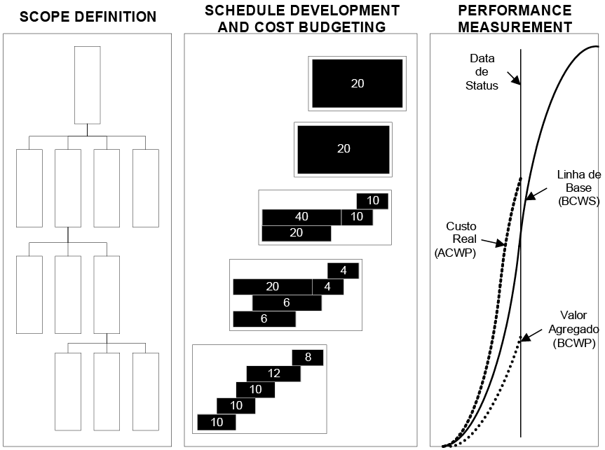Exhibit 1 – Planning and monitoring system using Earned Value Analysis (ABBA, 1998).

Likewise, the PMI (2000) shows, in its process of planning (Exhibit 2), a detailing of processes of planning according to the same steps mentioned by ABBA (1998), in which the scope definition of the project (Scope Definition – 5.3) is prerequisite for schedule development (Schedule Development – 6.4), for resource allocation (Resource Planning – 7.1) and for cost budgeting (Cost Budgeting – 7.3). Based on the conclusion of these processes, the project plan is developed (Project Plan Development – 4.1).

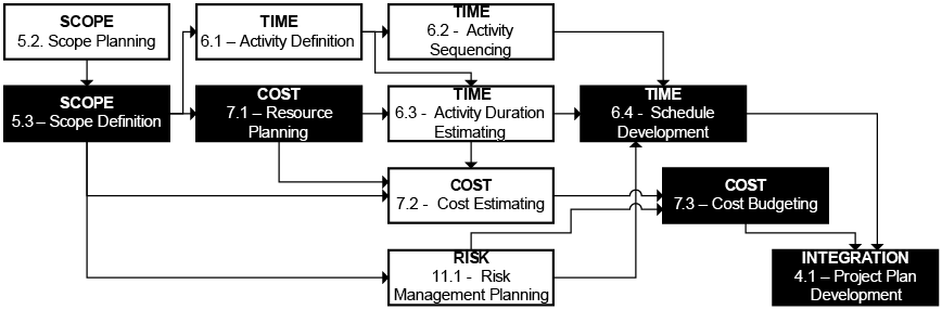Exhibit 2 – Planning processes (PMI,2000).

BCWS (Budget cost of work scheduled) is the value that points out the part of the budget that should be spent, considering the cost of baseline of the activity, attribution or resource. The BCWS is calculated as the costs of baseline divided in phases and accumulated until the date of the status, or current date. It is the cost originated in the budget.

During the execution, the monitoring of the progress of the project is made through the comparison between the real results obtained and the ones forecasted by the project in the BCWS. In this moment, the Earned Value of the work (BCWP) is evaluated, as well as the appropriation of real costs (ACWP).

BCWP (Budget cost work performed) is the value that points out the part of the budget that should be spent, considering the work done up to the moment and the cost of baseline for the activity, attribution or resource. The BCWP is also called Earned Value.

The way of measurement of Earned Value, or BCWP, is directly linked to the way the project was planned. Without an adequate planning, the measurement of performance has little or no applicability.

HARROFF (2000) and FLEMING & KOPPELMAN (1999) subdivide the measurement of Earned Value (BCWP) in different methods:

1. 1. Milestone with weighted value: The control cell is converted in 2 or more marks where each one of them is defined by a partial delivery of the work, generating, consequently, a specific cost. The sum of the costs of accomplishment of each one of these marks is the cost of the item.
2. 2. Fixed formula by CAP: It is the method that divides CAP in 2 parts that, if summed up, complete 100% of the work. In general, the most used formulas are 25/75, 50/50 and 75/25. The formula 25/75 separates the work in 2 points: the first point is accomplished immediately at the beginning of CAP (25% of costs are already accounted); the other 74% are accounted when the work is finished. The formula 50/50 points out that 50% of costs will be accounted at the beginning of the work and 50% at the end.
3. 3. Percent complete: This method attributes to each element of a certain percent complete (between 0 and 100%) to each control cycle. This percentage is multiplied by the forecasted cost, aiming to determine the part of the budget already done.
4. 4. Equivalent units: It is a method that calculates the Earned Value based on the units produced or made by individual elements of costs, applied in repetitive works or where the elements are defined in terms of direct consumption of resources.

It is common sense in all Earned Value reports that there is not only one method able to fulfill all kinds of work. Most of the times, companies should allow the use of more than a mechanism of Earned Value calculation.

In this article we decided to choose the use of percent complete as a way to determine Earned Value (BCWP), due to its popularity and user-friendliness. The percent complete is being more used in projects because it is easy to use and it is a standard entry mechanism for earned values in many project management software.

On the other hand, it brings a huge obstacle in its use, which is the strong subjectivity in its evaluation. It is influenced directly by the evaluator’s perception. Since the data entry relies on the individual perception, the percent complete method can be threatened by clients’ pressure or by management staff, and as a consequence it could harm the results obtained. In order to minimize those problems, some companies have been using internal evaluation procedures of percent complete. The use of Earned Value in projects leads to more precise estimates.

The actual costs (ACWP) are measured and evaluated by the project team that is in charge of accounts payable and receivable or by the finance department of the same company. The team is supposed to report the real cost of the project until the dead line (status) in a specified accounts plan, defined by the controller’s department of the enterprise.

ACWP (Actual cost of work performed) presents the actual costs resulting from the work already done by a resource or activity, until the status date, or actual date of the project, due to financial data. When those 3 parameters are defined, the analysis of results is obtained based on the correlation among the values found for each one of them in a certain status date.

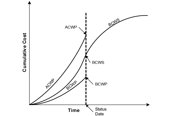Exhibit 3 – Graphic example of BCWS, BCWP and ACWP within a time length.

Project Evaluation and Development of Projections with the Earned Value Analysis

The correlation among the values of BCWS, BCWP and ACWP allows the verification of the results of the project and continue the evaluations and future projections of final costs

In order to relate between BCWP and the parameters BCWS and ACWP there are the following indexes:

A) SPI (Schedule Performance Index) – Division between the Earned Value (BCWP) and the planned value in the baseline (BCWS). The SPI shows the conversion rate of the forecasted value in Earned Value.

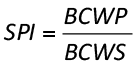(equation 01)

When the SPI equals 1 it means that the planned value was integrally earned to the project. When the SPI is less than 1 it means that the project is being done in a lower conversion rate than the forecasted one. In other words, the forecasted financial amount to be earned in the period defined couldn’t be obtained, and the project is late. When the SPI is superior to 1, it means that the project is earning results faster than expected, in other words, it is advanced.

B) CPI (Cost Performance Index) – Division between the Earned Value (BCWP) and the actual cost (ACWP). The CPI indicates which the conversion is between the actual values used by the project and the earned values in the same period.

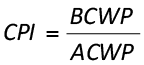(equation 02)

When the CPI equals 1, it means that the value spent by the project was integrally earned to the project (project within the budget). When the CPI is less than 1, it means that the project is spending more than forecasted until that moment. If the CPI is superior to 1, it means that the project costs less than forecasted until that moment. When CPI equals 1, it means that the project is according to the forecasted budget until the reference date. According to project forecasting, the following terminology is used:

A) EAC (Estimated at Completion) – finance value that represents the final cost of the project when concluded. It includes the actual costs (ACWP) and the rest of estimate values (ETC)

(equation 03)

B) ETC (Estimated to Complete) – financial value necessary to complete the project. It is calculated according to mathematical models to be presented.

C) VAC (Variation at Completion) – difference between the budgeted cost (BAC) and the projected final cost (EAC).

(equation 04)

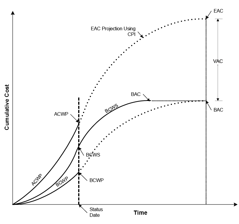Exhibit 4 – Earned Value forecasting of final deadlines and final costs (GEROSA & CAPODIFERRO, 1999).

Indexes Used for Projection of Project Final Costs

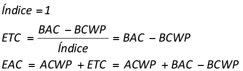
The generic formula for the remaining estimated cost is function of a performance factor

(equation 05)

where BAC is the final budget of the final project and index is the performance index of the project.

The performance index is determined by the combination of the Cost Performance Index (CPI) with the Scheduled Performance Index (SPI), according to what is described next, in its usual cases.

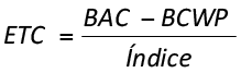
ETC through the constant deviation index (optimistic)

It assumes that the rest of the work to be done by the project will be done according to the original plan and that an occurred deviation will not represent a tendency of degeneration or recovery of the forecasted budget.

This estimate is commonly called the Optimistic Estimation, because, the indexes CPI and SPI are usually less than 1, therefore permanence in the plan turns out to be a good result.

(equation 06)

ETC through costs performance index (realistic or more probable)

It assumes that the rest of the work to be done by the project will follow the same finance performance obtained until this moment, through the costs performance index (CPI).

A negative or positive tendency obtained up to the moment in terms of CPI, will project the same tendency for the final costs of the project. Since, there is a natural tendency to work with CPI indexes inferior to 1, this estimate is commonly called Realistic Estimation or more probable.

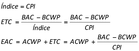(equation 07)

ETC through future scheduled cost index SCI (pessimistic)

It assumes that the rest of the work (future) to be done by the project will follow the finance projection determined by the cost performance index (CPI), as well as the scheduled projection determined by the scheduled performance index, generating the scheduled cost index SCI.

This procedure aims to catch a natural human tendency of recovering the time wasted, and this try means to spend more resources to do the same work planned before. The SCI index is strongly applicable in EAC projection in case of late projects, and with forecasted costs overspent. The product SPIxCPI makes up the strictest index in order to determine the EAC.

Since there is a natural tendency to work with CPI and SPI indexes inferior to 1, this estimate is usually called Pessimistic Estimation.

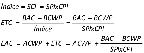(equation 08)

When the 3 ways of Estimated at completion is determined, a probabilistic model is applied in the data, in order to allow verification, in a desired reliability degree, which is the projected final cost for the project.

Monte Carlo Simulation

“Monte Carlo” was a nickname of a top-secret project related to the drawing and to the project of atomic weapons developed by the mathematician John von Neumann. He discovered that a simple model of random samples could solve certain mathematical problems, that couldn’t be solved up to the moment.

The simulation refers, however, to a method in which the distribution of possible results is produced from successive recalculations of the data of the project, allowing the construction of multiple scenarios. In each one of the calculations, new random data is used to represent a repetitive and interactive process. The combination of all these results creates a probabilistic distribution of the results.

The feasibility of produced distribution relies on the fact that, for a high number of repetitions, the model produced reflects the characteristics of the original distribution, transforming the distribution in a plausible result for analysis. The simulation can be applied in schedules, costs and other project indexes.

Mathematically the result of the simulation becomes a reasonable approximation for the original data. In an infinite number of repetitions, we could define that

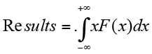(equation 09)

where X is the variable analyzed and F is its density of probabilities function.

Since the exact determination of the integration xF(x) is rather complex, the simulations permits an approximate form of results with less complexity.

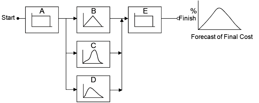Exhibit 5 – Construction of model of distribution of costs and activities or work packages making up a final distribution from random data of the project (PRITCHARD, 2001).

Execution of the Simulation

The execution of the simulation assumes that all data of SPI, CPI and EAC’s have already been determined for each activity or work package, according to what was evidenced in the project example shown as follows.

1 In this paper all the case study data are displayed in Brazilian Portuguese, as the original article.

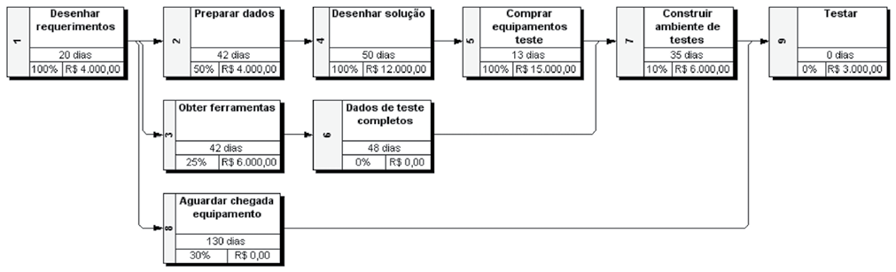Exhibit 6 – Project example using the simulation.1

From a complete database, the function of distribution of probability is determined for the 3 EAC data, building the medium EAC as a result of distribution, as shown at table below.

The function of density of probability used in the simulation will be the triangular distribution. This distribution is determined based on its minimum value, its more probable value and its maximum value. This function is probably the most direct and simplest among distributions (GREY, 1995), requiring only 3 points in its built.

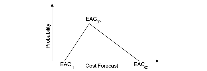
Exhibit 8 – Function of density of triangular probability for EAC.

Using the simulation software @Risk, we could determine the final EAC from the function RiskTriang (EAC1, EAC cpi, EAC sci), making up the results evidenced at table below.

When we build the function of density of probability, the parameters of simulation are determined, as well as the number of iterations and repetitions of simulation and other information. In this article 50,000 iterations were made.

The number of iterations is important to determine the quality of the results, therefore, the more iterations are made, the more the function of final density gets closer to the original functions. However, this kind of process requires a long execution time, even for fast computers that are able to make the simulation in high speed.

Analysis of the Results

After doing the simulation, the product generated is a distribution of probability of final EAC of the project, called “Simulation”, evidenced in the following exhibits.

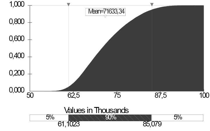Exhibit 11 – Distribution for the final EAC of the Project “Simulation” with an interval of confidence of 90% and cumulative distribution for the final EAC of the Project “Simulation”.

According to prior data, we can assume for sure (about 90% of certainty), for example that the projected final cost will be between $61,102 and $85,078.

These intervals could be altered in order to determine more or less precision. For example, assuming a certainty of 99% regarding the values, we obtain the interval between $57,858 and $90,792, according to what is shown in the following exhibit.

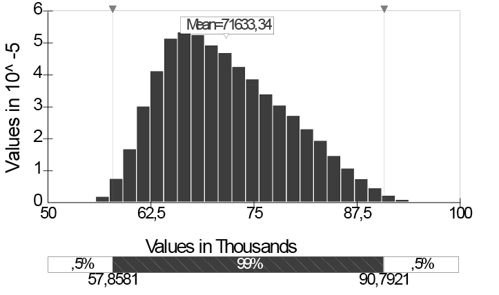Exhibit 13 – Distribution for the final EAC of the Project “Simulation” with an interval of confidence of 99%.

Conclusions

The use of Simulation Monte Carlo with the data of final EAC of the project, can, in an associated way, contribute to a probabilistic vision and not a deterministic vision of the final costs elaborated for the project, without the additional effort in its construction.

As mentioned in the study of CHRISTENSEN (1993), there isn’t an agreement in order to define which forecast model presents the best precision and applicability. However, many studies have been made in order to compare many models for the costs estimated in a certain project or group of projects, after its conclusion, aiming to identify which models are more precise and in which phases of the project they are applicable, as well as to associate a certain type of project to a certain index.

The need of estimates and costs projections is mentioned and characterized by DOD (1997) in Instruction 5000.2R in 1997 in 2 criterion.

Start with an estimate area for the final cost, reflecting the best and worst scenarios.(DOD, 1997).

Determine the estimate for the final cost that reflects the best professional judgment concerning costs. If the contract is at least 15% complete and the estimate is less than the calculated using the accumulated performance index, give an explanation (DOD, 1997).

However, none of these studies provides a probabilistic treatment for the projects, since the most adequate final EAC for the project is no longer an isolated value and turns out to be a values area with certain probabilities, as suggested in this article.

As a suggestion for new works, the next step will be to evaluate the results produced in the simulation with the real results of concluded projects in order to determine the precision of data obtained, aiming to produce cases associated to the simulation model applied to EMVS.

Abbreviations

ACWP – Actual cost of work performed

BAC – Budget at completion

BCWP – Budget cost of work performed

BCWS – Budget cost of work scheduled

C/SCSC – Cost/Schedule Systems Control Criteria

CAPs – Cost Account Plans

CPI – Cost Performance Index

CV – Cost variation

DOD – United States of America Department of Defense

EAC – Estimated at completion

EMVS – Earned Value Management Systems

ETC – Estimated to complete

EVMS – Earned value Analysis

PMBOK® – A guide to the Project Management Body of Knowledge

PMI – Project Management Institute

SCI – Scheduled Cost Index (SPIxCPI)

SPI – Scheduled Performance Index

SV – Scheduled variation

VAC – Variation at completion

References

ABBA, W. F. (1998). Defense Acquisition Reform and Project Management. Long Beach: 29th Annual Project Management Institute Seminars & Symposium.

CHRISTENSEN, D. S. (1993). Determining an Accurate Estimate at Completion. Vienna: National Contract Management Journal.

DOD (1997). Earned Value Management Implementation Guide. Washington: United States of America Department of Defense

FLEMING, Q. W. & KOPPELMAN, J. M. (1999). Earned value Project Management, 2nd Ed. Newton Square: Project Management Institute.

GEROSA S. & CAPODIFERRO C. (1999). Earned value Management (EMV) Techniques form Engineering and Prototype Production Activities. Philadelphia: 30th Annual Project Management Institute Seminars & Symposium.

GREY, S. (1995). Practical Risk Assessment for Project Management. West Sussex: John Wiley & Sons.

HARROFF, N. N. (2000). Discrete Versus Level of Effort. Milford: NNH Enterprise.

PMI (2000). A guide to the Project Management Body of Knowledge. Newton Square: Project Management Institute.

PRITCHARD, C. L. (2001). Risk Management: Concepts and Guidance. 2ª Ed. Arlington: ESI International.

SCHUYLER, J. R. (1994). Decision Analysis in Projects: Monte Carlo Simulation. Upper Darby: Project Management Institute.