The Planning Break-Even Point: When More Planning Stops Paying Off
Publications
PM World Journal
Addison, Texas, USA – November 2026
Ricardo Viana Vargas, Ph.D.
Carlos Augusto Freitas, MSc
1. Introduction
Most project managers have heard that time spent planning is time saved later, an old idea that is mostly right. A project that starts without clear requirements, a realistic schedule or a view of its main risks tends to pay for it during execution, usually in the form of rework. The same managers have also seen the opposite problem, with plans that keep growing, approval cycles that delay the start and teams that spend weeks refining documents that will change as soon as the work begins. Both failures are expensive, and the question that remains open in practice is where one ends and the other begins.
Research supports both sides of this argument. Dvir, Raz and Shenhar (2003) studied more than 100 defence research and development projects and found that success was positively correlated with the investment in requirements definition and technical specifications, while it was insensitive to the level of formal management procedures. Serrador and Turner (2015), with data on 1,386 projects, found an inverted-U relationship between planning effort and project success: projects can spend too little time planning, and they can also spend too much. Boehm (2002) framed the same question for software as a balance between two risks, in which too little planning leaves gaps that cause losses later and too much planning simply loses time.
In our view, what practitioners still lack is a simple way to put numbers on this balance for their own projects, and this paper is an attempt to offer one. Its starting point is a break-even rule first drafted by the second author, G ≤ R × P, which we extend into a model that finds both the optimal planning effort and the point where planning starts to destroy value.
The objective of this paper is to present, discuss and apply that model. It is not the scope of this paper to prove that planning improves project results, since the literature reviewed in Section 2 already supports that view, nor to propose benchmark values of planning effort by industry. The two cases in Section 5 use illustrative parameters, chosen to be plausible, to show how the model works and how sensitive its answers are.
After a review of the literature on planning, rework and planning effort in Section 2, the model is presented in Section 3 and the method used to apply it in Section 4. Section 5 applies the model to a software project and to an electrical substation project, Section 6 discusses the results, their practical use and their limitations, and Section 7 concludes.
2. Background
2.1 Planning and project success
Projects are temporary organizations that deliver something new under uncertainty and time pressure (Turner and Müller, 2003), and planning is the main way a team reduces that uncertainty before it commits most of the resources. The evidence that planning matters is strongest for the early definition of the work. In the study by Dvir, Raz and Shenhar (2003), what mattered was the effort spent on defining requirements and technical specifications, not the amount of procedure. In capital projects, research on more than 200 projects worth about US$8.7 billion showed a positive relationship between thorough pre-project planning and project performance (Gibson et al., 2006). Merrow (2011) reports that the quality of front-end loading is the most reliable predictor of the results of industrial megaprojects. Flyvbjerg and Gardner (2023) summarize the same lesson as "think slow, act fast": planning is relatively cheap and safe, while delivery is where money and risk concentrate.
2.2 Rework as the price of insufficient planning
Rework is the most direct cost of planning too little. In software, Boehm and Basili (2001) estimated that current projects spend about 40 to 50 percent of their effort on avoidable rework. In construction, Love (2002) found in 161 Australian projects that rework accounted for 52% of cost growth. In a later study, Love and Edwards (2005) reported mean direct and indirect rework costs of 6.4% and 5.9% of contract value. Hwang et al. (2009) analysed 359 projects from the Construction Industry Institute database and found that direct field rework in owner-reported projects averaged from about 4% of construction-phase cost in heavy industrial projects to about 9% in light industrial projects.
This literature shapes the model in Section 3 in two ways. Because rework varies so much between sectors and between projects, the model has to let the user set the rework level for the project at hand. And because rework costs more than the hours spent redoing the work (materials are scrapped, equipment is handled twice and delays can trigger penalties), the model also needs a way to price a rework hour above its labour cost. The indirect costs reported by Love and Edwards (2005), of the same order as the direct ones, suggest that this is far from a detail.
Studies of project failure are often quoted to justify more planning. The best known is the CHAOS report, which stated that 31.1% of software projects would be cancelled and that 52.7% would cost 189% of their original estimates (Standish Group, 1995). The method behind these figures has been criticized (Jørgensen and Moløkken-Østvold, 2006; Eveleens and Verhoef, 2010), and this paper does not use them to set any parameter.
2.3 How much planning is enough?
Boehm (2002) asked this question directly. He treated planning as a risk management decision: a small planning investment leaves a high probability of loss-causing gaps in the plan, while a large investment loses time that the project and its market may not have. The total risk exposure is lowest at a "sweet spot" between the two. Boehm and Turner (2003; 2004) used this logic to decide how much plan-driven discipline and how much agility a project needs.
Serrador and Turner (2015) gave the question its strongest empirical answer so far. In their global sample, the share of effort spent on planning that maximized project success was about 25% of total project effort, well above the 15% average reported by respondents. Serrador (2015) develops these findings for practitioners. The effects were strongest on overall success and weaker on efficiency measures such as time and budget.
Practice adds two further ideas to this discussion. Rolling wave planning spreads the planning effort over the life cycle, detailing near-term work and leaving later work at a lower level of detail (Githens, 1998). When deadlines are tight, a short list of essential planning processes can replace a full plan (Vargas, 2011). Project Management Institute (2021) also treats planning as a performance domain whose depth should be tailored to the project. None of these sources, however, gives a manager a formula to estimate how much planning effort a specific project should receive.
2.4 Putting a value on project management
The model in this paper belongs to a line of work that turns qualitative claims about project management into numbers. Kwak and Ibbs (2000) proposed ways to calculate the return on investment of project management. Vargas (2013) used Monte Carlo simulation to estimate the return of a project management implementation, and Vargas (2004) used it to turn earned value forecasts into probability ranges. Hubbard (2010) argues that any quantity becomes measurable once it is seen as a reduction of uncertainty. The same approach is used here: the claim that "planning saves money" becomes an estimate with a range around it.
3. The model
3.1 Definitions and assumptions
Table 1 lists the variables. All efforts are expressed as shares of the baseline effort T, and all costs as shares of the baseline labour cost C × T. This makes the results independent of project size and currency.
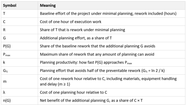
Table 1: Model variables
The model rests on four assumptions.
- The baseline is minimal planning, not zero planning. Every real project does some planning, and G measures only the effort added on top of that minimum.
- The only benefit counted is avoided rework. Planning also improves stakeholder alignment, scope definition, procurement and team motivation. These benefits are real but harder to price, so leaving them out makes the model conservative.
- A planning hour costs λ × C and a rework hour costs m × C. In the base case m = λ = 1.
- The model works with effort, not calendar time. Effects on duration, such as a later market entry or a delay penalty, can be added through m or λ (Section 6).
3.2 The break-even rule
If planning avoids a constant share P of the rework, the net benefit of an additional planning effort G is the rework cost avoided minus the cost of the planning:
N(G) = m · C · T · R · P − λ · C · T · G (1)
Dividing by the baseline labour cost C × T gives the net benefit as a share of that cost:
n(G) = m · R · P − λ · G (2)
Planning pays for itself when n(G) ≥ 0, that is, when
G ≤ m · R · P / λ (3)
With m = λ = 1 this is the original rule, G ≤ R × P. If rework takes 30% of the baseline effort and planning avoids 70% of it, planning pays for itself as long as it uses no more than 21% of the baseline effort.
The rule, however, has a weakness that becomes clear when equation (2) is plotted (Figure 1). If P does not depend on G, the net benefit falls in a straight line from G = 0, and the model, read literally, recommends the smallest plan that still achieves P. In other words, the rule answers an average-return question, whether the plan as a whole pays for itself, but it cannot answer the marginal question that managers face every week, which is whether to plan for one more week. For that, P must depend on G.
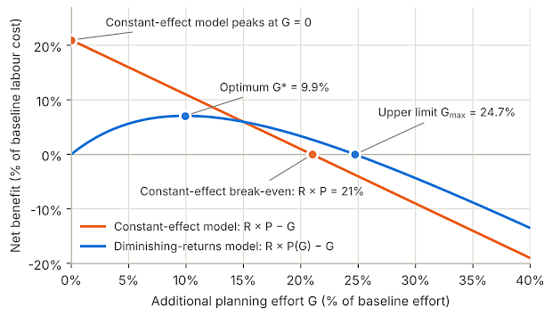
Figure 1: Net benefit under the constant-effect rule and under diminishing returns (Case B parameters)
3.3 Adding diminishing returns
The first hours of planning remove the most rework, because they settle objectives, scope, critical interfaces and the main risks, while later hours refine details that are more likely to change anyway. Some rework can never be prevented, because it comes from events no plan can foresee, such as regulatory changes, market shifts or late decisions by the customer. The simplest curve with these two properties is
P(G) = Pmax · (1 − e−k · G) (4)
The net benefit becomes
n(G) = m · R · Pmax · (1 − e−k · G) − λ · G (5)
The optimal planning effort G* is the point where one more unit of planning avoids exactly as much rework cost as it costs:
m · R · Pmax · k · e−k · G* = λ (6)
This means that a team should keep planning while the next hour of planning avoids more than λ / m hours of rework. Solving equation (6) gives
G* = (1 / k) · ln(m · R · Pmax · k / λ) (7)
Equation (7) is valid when m · R · Pmax · k > λ. Otherwise, even the first hour of extra planning does not pay, and G* = 0. The net benefit at the optimum is
n(G*) = m · R · Pmax − λ / k − λ · G* (8)
The upper limit Gmax is the planning effort above G* at which the net benefit returns to zero:
n(Gmax) = 0, with Gmax > G* (9)
Equation (9) has no solution in elementary functions, but any spreadsheet can solve it with a goal-seek function. The search should start above G*, for example at m · R · Pmax / λ, because n(G) is also zero at G = 0.
3.4 Two simple bounds
The model gives two bounds that a manager can use even before estimating k. Because P(G) is always below Pmax, the net benefit is always below m · R · Pmax − λ · G. Planning effort above m · R · Pmax / λ therefore always destroys value:
Gmax < m · R · Pmax / λ (10)
The second bound comes from asking how G* changes with the planning productivity k. Writing a = m · R · Pmax / λ, equation (7) becomes G* = ln(a · k) / k. Its derivative with respect to k is (1 − ln(a · k)) / k², which is zero when a · k = e, Euler's number (about 2.718). At that point G* = 1 / k = a / e, which is the highest value G* can take. Therefore, whatever the planning productivity,
G* ≤ m · R · Pmax / (e · λ) ≈ 0.37 · m · R · Pmax / λ (11)
With m = λ = 1, the optimal additional planning effort is at most about 37% of the preventable rework R × Pmax. For R = 30% and Pmax = 90%, the optimum can never exceed 9.9% of the baseline effort, and planning above 27% always loses money. Table 2 brings the three rules together.
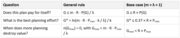
Table 2: Three rules for planning effort
4. Method
The model was applied to two illustrative cases: a software development project (Case A) and the construction of an electrical substation (Case B). The parameters are not records from real projects. They were chosen to be plausible for each type of project. Case A uses a rework level below the values reported for software in Section 2. Case B uses a level above the construction averages, for the reasons given in Section 5.2.
Practitioners rarely know the planning productivity k directly. It is easier for a team to answer a question such as "if we added 10% more planning effort, how much of the usual rework would we avoid?". One answer of this kind, a calibration point (Gref, Pref), fixes k:
k = −ln(1 − Pref / Pmax) / Gref (12)
Each case was analysed with a deterministic calculation of G*, Gmax, the net benefit and the effort in hours, using equations (4) to (9) and (12). This was followed by a one-at-a-time sensitivity analysis of G*, shown as a tornado chart, and by a Monte Carlo simulation with 10,000 iterations, following the approach used by Vargas (2004; 2013). In the simulation, R, Pmax and G½ were drawn from triangular distributions, with m = λ = 1 (Table 5). For each iteration we computed G*, n(G*), Gmax and the full net benefit curve. From these we obtained percentiles, the expected net benefit for each planning level and the probability that a given planning level pays for itself. The calculations were done in Python (NumPy and SciPy) with a fixed random seed, so the results can be reproduced. The deterministic results can also be reproduced in a spreadsheet with equations (4) to (9) and (12).
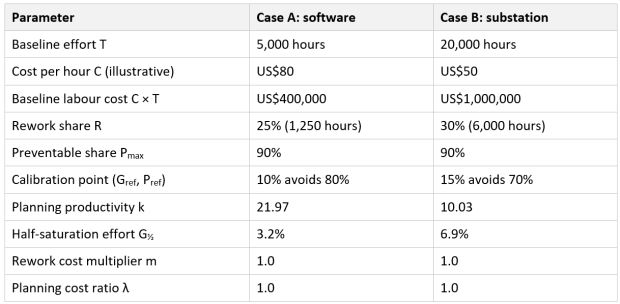
Note: In Case B, C × T covers labour only. Equipment and materials are excluded, which is why the baseline labour cost is far below the total cost of a substation.
Table 3: Parameters of the two cases
5. Results
5.1 Case A: software development project
The software project has a baseline effort of 5,000 hours, of which 25%, or 1,250 hours, is rework. This is a conservative value, well below the 40% to 50% of avoidable rework reported by Boehm and Basili (2001). The team estimates that 10% of additional planning would avoid 80% of the rework.
The break-even rule confirms that this plan pays for itself, since 10% is below R × P = 25% × 80% = 20%. The net benefit of the plan is 10% of the baseline labour cost, or US$40,000, but the plan is not the best one available, since the optimum is G* = 7.3%, or 364 hours of additional planning. At that level, planning avoids 71.8% of the rework (897 hours), the total effort falls from 5,000 to 4,466 hours, and the net benefit is 10.7% of the baseline labour cost, or US$42,700. The bound in equation (11) is 25% × 90% / e = 8.3%, so the optimum sits just below its ceiling.
Near its peak the net benefit curve is quite flat, and planning 5% or 10% gives almost the same result as the optimum, about 10%. Beyond 15% the curve falls quickly: at 20% of additional planning the net benefit is down to 2.2%, and at Gmax = 22.3% (1,117 hours) it reaches zero, so that every hour of planning beyond that point costs more than the rework it removes.
5.2 Case B: electrical substation project
The substation project has a baseline effort of 20,000 hours, with 30% of rework, or 6,000 hours. This value is higher than the construction averages in Section 2 because the baseline is minimal planning and the rework is measured in labour hours, which include the repeated installation, testing and commissioning work. The team estimates that 15% of additional planning would avoid 70% of the rework.
The break-even rule confirms that the plan pays for itself (15% is below 30% × 70% = 21%), with a net benefit of 6%, or US$60,000 and 1,200 hours. Here too the optimum is lower, at G* = 9.9%, or 1,987 hours of additional planning. Planning at this level avoids 56.8% of the rework (3,405 hours), the total effort falls to 18,581 hours, and the net benefit is 7.1% of the baseline labour cost, or US$70,900 and 1,419 hours. In this case G* coincides with the bound of equation (11), 30% × 90% / e = 9.9%, because the calibration point places k very close to the value that maximizes G*. The upper limit is Gmax = 24.7% (4,948 hours), below the ceiling of 27% given by equation (10).
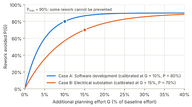
Figure 2: Rework avoided as a function of additional planning effort, with the calibration points of each case
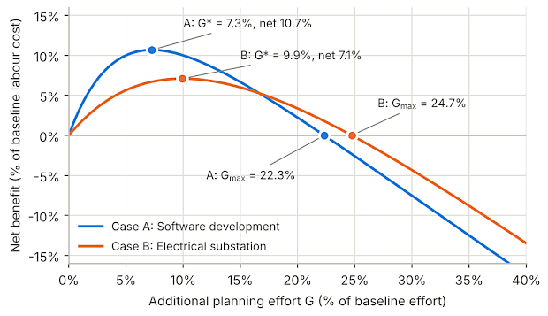
Figure 3: Net benefit of additional planning in the two cases, with the optimum G* and the upper limit Gmax
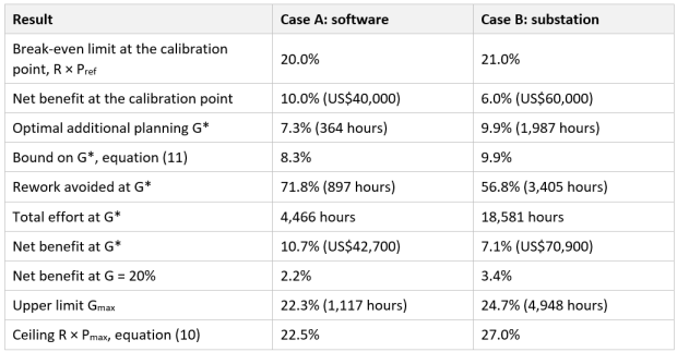
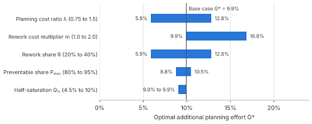
Figure 4: Sensitivity of the optimal additional planning effort G* to each parameter (Case B)
5.4 Monte Carlo simulation
Table 5 shows the distributions used in the simulation and Table 6 the main results. In both cases the optimum stays within a narrow band. The 10th to 90th percentile range of G* is 6.1% to 9.3% in Case A and 5.4% to 11.2% in Case B. The planning level with the highest expected net benefit is 7.7% in Case A (expected net benefit 10.3%) and 8.9% in Case B (5.2%).

Table 5: Distributions used in the Monte Carlo simulation (triangular: minimum, mode, maximum)
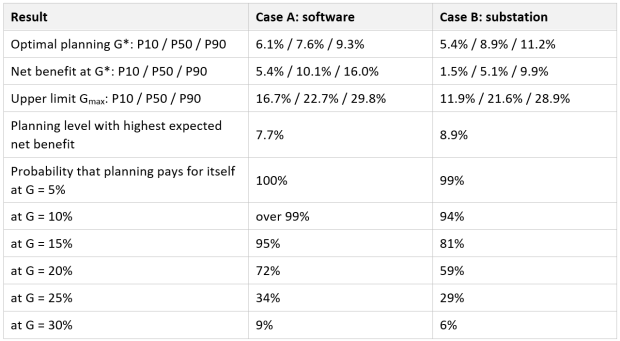
Table 6: Monte Carlo results, 10,000 iterations (P10, P50 and P90 are the 10th, 50th and 90th percentiles)
The simulation also shows that the two kinds of error behave differently (Figure 5). A plan below the optimum gives up part of the benefit but still pays for itself. In the model the net benefit is positive for any planning effort between zero and Gmax, and at 5% of additional planning the probability that planning pays for itself is 100% in Case A and 99% in Case B, with an expected net benefit of 9.4% and 4.4%, against 10.3% and 5.2% at the best level. A plan far above the optimum can lose money, and the loss grows with every extra hour of planning. At 20% of additional planning, the probability that the plan pays for itself drops to 72% in Case A and 59% in Case B. At 25% it falls to 34% and 29%.
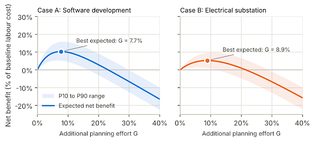
Figure 5: Expected net benefit and 10th to 90th percentile range from the Monte Carlo simulation
6. Discussion
6.1 What the model says about the break-even rule
In our view the rule G ≤ R × P should be used as a test and not as a target. When the team can estimate how much rework a given plan avoids, the rule tells whether that plan pays for itself; used as a target, it leads to a plan whose net benefit is, by construction, zero. In both cases the optimum was well below the break-even limit: 7.3% against 20% in Case A, and 9.9% against 21% in Case B. Equation (11) gives a quick way to see why, since with m = λ = 1 the optimum can never exceed about 37% of R × P
6.2 Comparison with empirical evidence
The optimum found here, between 7% and 10% of additional effort, is lower than the 25% of total effort that maximized success in the study by Serrador and Turner (2015). The difference is less of a contradiction than it may seem, because the two numbers do not measure the same thing. Our G is the effort added on top of a minimal plan, whereas their figure is the total planning effort, minimum included. The model also counts only avoided rework, while their study measured overall success, including stakeholder satisfaction and benefits, and it found weaker effects of planning on efficiency measures such as time and budget, which are the closest to what this model counts. The result also depends heavily on the cost of rework beyond labour hours, and with m = 2 the optimum in Case B rises to 16.8%.
For these reasons the G* computed by this model should be read as a conservative estimate: if planning brings other benefits that grow with planning effort, the true optimum is higher than G*. On the direction, at least, the model and the empirical evidence agree. Most projects can gain from somewhat more planning than the minimum, and there is a point beyond which more planning loses value.
6.3 Practical use for project managers and PMOs
A project manager can apply the model in five steps.
- Estimate the rework share R from lessons learned, change logs and quality records of similar projects. Teams tend to be optimistic about their own projects (Lovallo and Kahneman, 2003), so historical data is better than opinion.
- Estimate the preventable share Pmax by classifying past rework by root cause and separating what better planning could have prevented from what it could not.
- Agree on a calibration point with the team, for example "with 10% more planning we would avoid 80% of the usual rework". Expert judgement, the Delphi technique or pairwise comparison with the analytic hierarchy process (Vargas, 2010) can support this estimate.
- Set the cost ratios: m for the non-labour cost of rework, such as materials, penalties and delay, and λ for the relative cost of planning hours.
- Compute G*, Gmax and the bounds in equations (10) and (11). Plan in rolling waves (Githens, 1998) and review the parameters at each phase gate, when the team knows more.
For a PMO, the model offers a common language for the decision. Instead of debating whether a plan is "too long", the sponsor and the team can discuss the parameters, which can be checked against records. Over time, a PMO that records rework and planning effort by project type can calibrate R, Pmax and k from its own portfolio and set planning guidelines for each type of project.
6.4 Limitations
Like any simplification of a complex environment, the model has limitations that the reader should keep in mind. The cases use illustrative parameters, so the numbers in Section 5 show how the model behaves and should not be taken as benchmarks. The exponential response curve is itself an assumption, and an S-shaped curve, in which the first planning hours carry a setup cost before they start to pay off, would tend to move G* to the right. Because the model works with effort and ignores calendar time, the cost of delay has to be added through m or λ wherever speed to market or a delivery date matters. Counting a single benefit, avoided rework, makes the model conservative, as discussed above. Real projects also plan in waves rather than through a single upfront decision, although the model can be applied to each wave separately. Finally, the Monte Carlo simulation treats R, Pmax and G½ as independent, while in practice a project with high rework may also have a high share of preventable rework.
7. Conclusions
This paper set out to answer a common question in project management: how much planning is enough? It started from a break-even rule, G ≤ R × P, and showed that the rule is a sound test of whether a plan pays for itself but not a guide to how much to plan. Adding diminishing returns produced a model with a closed-form optimum, G* = ln(m · R · Pmax · k / λ) / k, an upper limit Gmax, and two bounds that need no estimate of planning productivity. In the base case, the optimal additional effort never exceeds about 37% of the preventable rework, and planning beyond R × Pmax always loses money.
In two illustrative cases, a software project and an electrical substation, the optimum was between 7% and 10% of the baseline effort and saved between 7% and 11% of the baseline labour cost. Planning above 22% to 25% destroyed value. In the Monte Carlo simulation, the optimum stayed between about 5% and 11% (10th to 90th percentiles) across the ranges of R, Pmax and G½ tested. The simulation also showed that a plan below the optimum gives up part of the benefit but still pays for itself, while a plan above the upper limit loses money, and the loss grows with every extra hour of planning. The optimum depends mostly on the size and cost of rework and on the cost of planning hours. The effect of planning productivity is smaller near the calibrated values and is always capped by the bound in equation (11).
It is important to highlight that the model does not replace the judgement of the project manager and the sponsor. What it offers is a shared and explicit way to discuss how much planning a project needs, and to revisit that decision as the project learns. Future research should calibrate the model with real data from project portfolios, test other response curves and include the effect of planning on project duration.
Declaration on the use of artificial intelligence
The authors used Claude (Anthropic, Claude Opus 5.5) to review and proofread the English translation of the original Portuguese manuscript, focusing on grammar, clarity, and language. No images were generated or created using AI. The authors reviewed and verified all content and take full responsibility for the final text and its accuracy.
References
Boehm, B. (2002) 'Get ready for agile methods, with care', Computer, 35(1), pp. 64-69. doi:10.1109/2.976920.
Boehm, B. and Basili, V.R. (2001) 'Software defect reduction top 10 list', Computer, 34(1), pp. 135-137. doi:10.1109/2.962984.
Boehm, B. and Turner, R. (2003) 'Using risk to balance agile and plan-driven methods', Computer, 36(6), pp. 57-66. doi:10.1109/MC.2003.1204376.
Boehm, B. and Turner, R. (2004) Balancing agility and discipline: a guide for the perplexed. Boston, MA: Addison-Wesley.
Dvir, D., Raz, T. and Shenhar, A.J. (2003) 'An empirical analysis of the relationship between project planning and project success', International Journal of Project Management, 21(2), pp. 89-95. doi:10.1016/S0263-7863(02)00012-1.
Eveleens, J.L. and Verhoef, C. (2010) 'The rise and fall of the Chaos report figures', IEEE Software, 27(1), pp. 30-36. doi:10.1109/MS.2009.154.
Flyvbjerg, B. and Gardner, D. (2023) How big things get done. New York: Currency.
Gibson, G.E., Wang, Y.-R., Cho, C.-S. and Pappas, M.P. (2006) 'What is preproject planning, anyway?', Journal of Management in Engineering, 22(1), pp. 35-42. doi:10.1061/(ASCE)0742-597X(2006)22:1(35).
Githens, G.D. (1998) 'Rolling wave project planning', Proceedings of the 29th Annual Project Management Institute Seminars & Symposium, Long Beach, CA. Newtown Square, PA: Project Management Institute.
Hubbard, D.W. (2010) How to measure anything: finding the value of "intangibles" in business. 2nd edn. Hoboken, NJ: Wiley.
Hwang, B.-G., Thomas, S.R., Haas, C.T. and Caldas, C.H. (2009) 'Measuring the impact of rework on construction cost performance', Journal of Construction Engineering and Management, 135(3), pp. 187-198. doi:10.1061/(ASCE)0733-9364(2009)135:3(187).
Jørgensen, M. and Moløkken-Østvold, K. (2006) 'How large are software cost overruns? A review of the 1994 CHAOS report', Information and Software Technology, 48(4), pp. 297-301. doi:10.1016/j.infsof.2005.07.002.
Kwak, Y.H. and Ibbs, C.W. (2000) 'Calculating project management's return on investment', Project Management Journal, 31(2), pp. 38-47.
Lovallo, D. and Kahneman, D. (2003) 'Delusions of success: how optimism undermines executives' decisions', Harvard Business Review, 81(7), pp. 56-63.
Love, P.E.D. (2002) 'Influence of project type and procurement method on rework costs in building construction projects', Journal of Construction Engineering and Management, 128(1), pp. 18-29. doi:10.1061/(ASCE)0733-9364(2002)128:1(18).
Love, P.E.D. and Edwards, D.J. (2005) 'Calculating total rework costs in Australian construction projects', Civil Engineering and Environmental Systems, 22(1), pp. 11-27. doi:10.1080/10286600500049904.
Merrow, E.W. (2011) Industrial megaprojects: concepts, strategies, and practices for success. Hoboken, NJ: Wiley.
Project Management Institute (2021) A guide to the project management body of knowledge (PMBOK guide) and the standard for project management. 7th edn. Newtown Square, PA: Project Management Institute.
Serrador, P. (2015) Project planning and project success: the 25% solution. Boca Raton, FL: CRC Press.
Serrador, P. and Turner, R. (2015) 'What is enough planning? Results from a global quantitative study', IEEE Transactions on Engineering Management, 62(4), pp. 462-474. doi:10.1109/TEM.2015.2448059.
Standish Group (1995) CHAOS. Boston, MA: The Standish Group.
Turner, J.R. and Müller, R. (2003) 'On the nature of the project as a temporary organization', International Journal of Project Management, 21(1), pp. 1-8. doi:10.1016/S0263-7863(02)00020-0.
Vargas, R.V. (2004) 'Earned value probabilistic forecasting using Monte Carlo simulation', AACE International 48th Annual Meeting, Washington, DC. Morgantown, WV: AACE International.
Vargas, R.V. (2010) 'Using the analytic hierarchy process (AHP) to select and prioritize projects in a portfolio', PMI Global Congress 2010, North America, Washington, DC. Newtown Square, PA: Project Management Institute.
Vargas, R.V. (2011) 'Urgency: a critical factor in project planning', PMI Global Congress 2011, North America, Dallas, TX. Newtown Square, PA: Project Management Institute.
Vargas, R.V. (2013) 'Determining the mathematical ROI of a project management implementation', PMI Global Congress 2013, North America, New Orleans, LA. Newtown Square, PA: Project Management Institute.
Access the original paper at https://pmworldjournal.com/article/the-planning-break-even-point